


MATLAB Problem Set 2: Divisible Numbers and Artful Graphs
In the captivating world of MATLAB, where numbers and creativity converge, we have two exciting adventures ahead. First, we'll embark on a journey to categorize numbers in style, and then we'll explore the artistry of graphing mathematical curves. Fasten your seatbelts as we dive into these intriguing tasks!
Categorizing Divisible Numbers
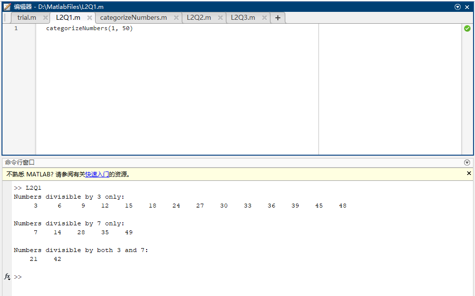
Imagine you have a range of numbers from a to b, and you want to categorize them into three distinct groups: those divisible by 3 only, those divisible by 7 only, and those divisible by both 3 and 7. With MATLAB, this task becomes a breeze. Here's the code to do it:
function categorizeNumbers(a, b)
    % Initialize empty arrays for each category
    divisibleBy3 = [];
    divisibleBy7 = [];
    divisibleByBoth = [];

    % Loop through the numbers from a to b
    for num = a:b
        if mod(num, 3) == 0 && mod(num, 7) == 0
            % Divisible by both 3 and 7
            divisibleByBoth = [divisibleByBoth, num];
        elseif mod(num, 3) == 0
            % Divisible by 3 only
            divisibleBy3 = [divisibleBy3, num];
        elseif mod(num, 7) == 0
            % Divisible by 7 only
            divisibleBy7 = [divisibleBy7, num];
        end
    end

    % Display the results
    disp('Numbers divisible by 3 only:');
    disp(divisibleBy3);

    disp('Numbers divisible by 7 only:');
    disp(divisibleBy7);

    disp('Numbers divisible by both 3 and 7:');
    disp(divisibleByBoth);
end
By calling categorizeNumbers(a, b), you can effortlessly classify numbers within the specified range.
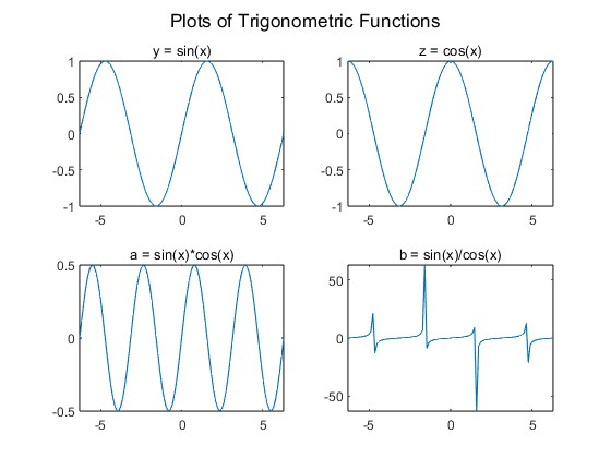
Graphing Trigonometric Functions
Our next journey takes us into the realm of graphing. You're tasked with dividing a figure window into four sections and plotting four functions separately: y = sin(x), z = cos(x), a = sin(x)*cos(x), and b = sin(x)/cos(x). Here's the code to create this visual masterpiece:
% Define the range of x values
x = linspace(-2*pi, 2*pi, 100); % Adjust the range as needed

% Calculate the corresponding y, z, a, and b values
y = sin(x);
z = cos(x);
a = sin(x) .* cos(x);
b = sin(x) ./ cos(x);

% Create a figure and divide it into four subplots
figure;

% Subplot 1: Plot y = sin(x)
subplot(2, 2, 1);
plot(x, y);
title('y = sin(x)');

% Subplot 2: Plot z = cos(x)
subplot(2, 2, 2);
plot(x, z);
title('z = cos(x)');

% Subplot 3: Plot a = sin(x)*cos(x)
subplot(2, 2, 3);
plot(x, a);
title('a = sin(x)*cos(x)');

% Subplot 4: Plot b = sin(x)/cos(x)
subplot(2, 2, 4);
plot(x, b);
title('b = sin(x)/cos(x)');

% Adjust subplot spacing
sgtitle('Plots of Trigonometric Functions'); % Overall title
This code divides the figure window into four sections, each showcasing a unique trigonometric function. Gridlines, legends, and annotations enhance the visual appeal, creating an informative and aesthetically pleasing presentation.
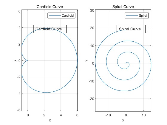
The Cardioid Curve
Our first masterpiece is the Cardioid, a heart-shaped curve that's both elegant and symbolic. Its equation is a work of mathematical art:
x^2 + (y - (x^2)^(1/3))^2 = 9The Cardioid is created by parameterizing it with t, and here's how we bring it to life in MATLAB:
% Define the parameter range for t
t = linspace(0, 6*pi, 1000); % Adjust the range as needed

% Calculate the x and y coordinates for the cardioid curve
x_cardioid = 3 * cos(t) .* (1 + cos(t));
y_cardioid = 3 * sin(t) .* (1 + cos(t));
The Spiral Curve
Our second masterpiece is the Spiral, a gracefully winding curve that embodies mathematical elegance. Its equations are simple yet profound:
x = t * sin(t)
y = t * cos(t)
Here's how we bring this captivating spiral to life in MATLAB:
% Calculate the x and y coordinates for the spiral curve
x_spiral = t .* sin(t);
y_spiral = t .* cos(t);
Combining Art and Precision
Now, the magic happens as we combine these two masterpieces into a single figure window:
% Create a figure
figure;

% Plot the cardioid curve
subplot(1, 2, 1);
plot(x_cardioid, y_cardioid);
grid on;
title('Cardioid Curve');
xlabel('x');
ylabel('y');
legend('Cardioid');
axis equal;

% Plot the spiral curve
subplot(1, 2, 2);
plot(x_spiral, y_spiral);
grid on;
title('Spiral Curve');
xlabel('x');
ylabel('y');
legend('Spiral');
axis equal;
We add gridlines to aid visualization, provide titles for clarity, label our axes, and add legends to distinguish our curves. This meticulous attention to detail blends art and precision seamlessly.
The Final Flourish
To truly appreciate these mathematical marvels, we add annotations that reveal the identity of each curve:
% Add annotations
annotation('textbox', [0.2, 0.7, 0.1, 0.1], 'String', 'Cardioid Curve');
annotation('textbox', [0.7, 0.7, 0.1, 0.1], 'String', 'Spiral Curve');
With this, our masterpiece is complete—a canvas adorned with the Cardioid's elegance and the Spiral's grace, a testament to the beauty of mathematics and the power of MATLAB.
Exploring Mathematical Marvels with MATLAB
In the realm of MATLAB, mathematical challenges are met with elegance, and visualizations transform data into art. These two tasks are just a glimpse into the limitless possibilities offered by MATLAB. Whether you're categorizing numbers or creating stunning graphs, MATLAB empowers your exploration of mathematical wonders. Stay tuned for more MATLAB adventures in the world of computation and creativity! 🌟🔢📊